While all my blog posts till now were kind of abstract, here I will try to show some of the technical details of the project without making it too bloated. So as a one-line description, I had to study, implement and integrate a spectral estimation technique, namely the Multitaper Periodogram³ (and its derivatives¹), which are used to analyze astronomical time series.

Why spectral representations?

Before getting into the how of spectral analysis and its estimation, a brief sidenote on the why. Why do we even bother to study the spectral properties of a time series? It turns out, some of the determining characteristics or defining parameters associated with a certain time series are better brought out in their spectral representations (frequency domain representations).

As an example, the power spectral density is a common tool to try and unearth the periodic element(s) in a time series. Such spectral analysis techniques, at their core, are enabled by the Fourier Transform, and if you’d like to gain a better intuitive understanding of it, do check out this awesome video by Grant Sanderson on 3Blue1Brown.

Multi what?

Spectral analysis isn’t without its fair share of practical complications, in fact, far from it. But there have been quite a few very effective techniques to mitigate them.

One of them is tapering (multiplying the time series with a bell-shaped function), effective in reducing spectral leakage. Tapering a time series as a way of obtaining a spectral estimator with acceptable bias properties is an important concept. The loss of information (contained at the extremes of the time series) inherent in tapering can often be avoided either by prewhitening or by using Welch’s overlapped segment averaging.

The multitaper periodogram is another approach to recover information lost due to tapering. This approach was introduced by Thomson (1982)³ and involves the use of multiple orthogonal tapers, having approximately uncorrelated spectral densities.

In the multitaper method, the data is windowed or tapered, but this method differs from the traditional methods in the tapers used, which are the most band-limited functions amongst those defined on a finite time domain, and also, these tapers are orthogonal, enabling us to average the eigenspectrum (spectrum estimates from individual tapers) from more than one tapers to obtain a superior estimate in terms of noise. The resulting spectrum has low leakage, low variance, and retains information contained in the beginning and end of the time series.

The tapers used are the discrete prolate spheroidal sequences (DPSS), or, the Slepians (Slepian 1978)⁴.

A look at the DPSS tapers

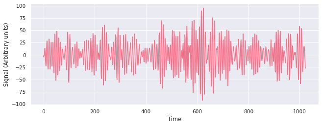
Let’s consider a time series sampled from an autoregressive process of order 4, AR(4), which has been frequently exemplified in literature¹ in similar contexts.

A good way to gain an intuitive understanding of the properties of the DPSS tapers, and how they affect the time series, is to visualize the effect. Given here are the time and frequency domain representations of the tapers and the tapered time series.

The first 8 tapers and the corresponding tapered time series⁵.

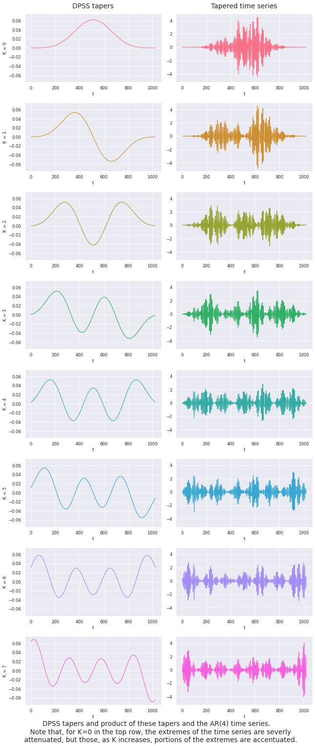
This showcases the product of a windowing function and a time series quite well. Next let’s have a look at their spectral representations⁵, more specifically, their power spectrum densities (PSD).

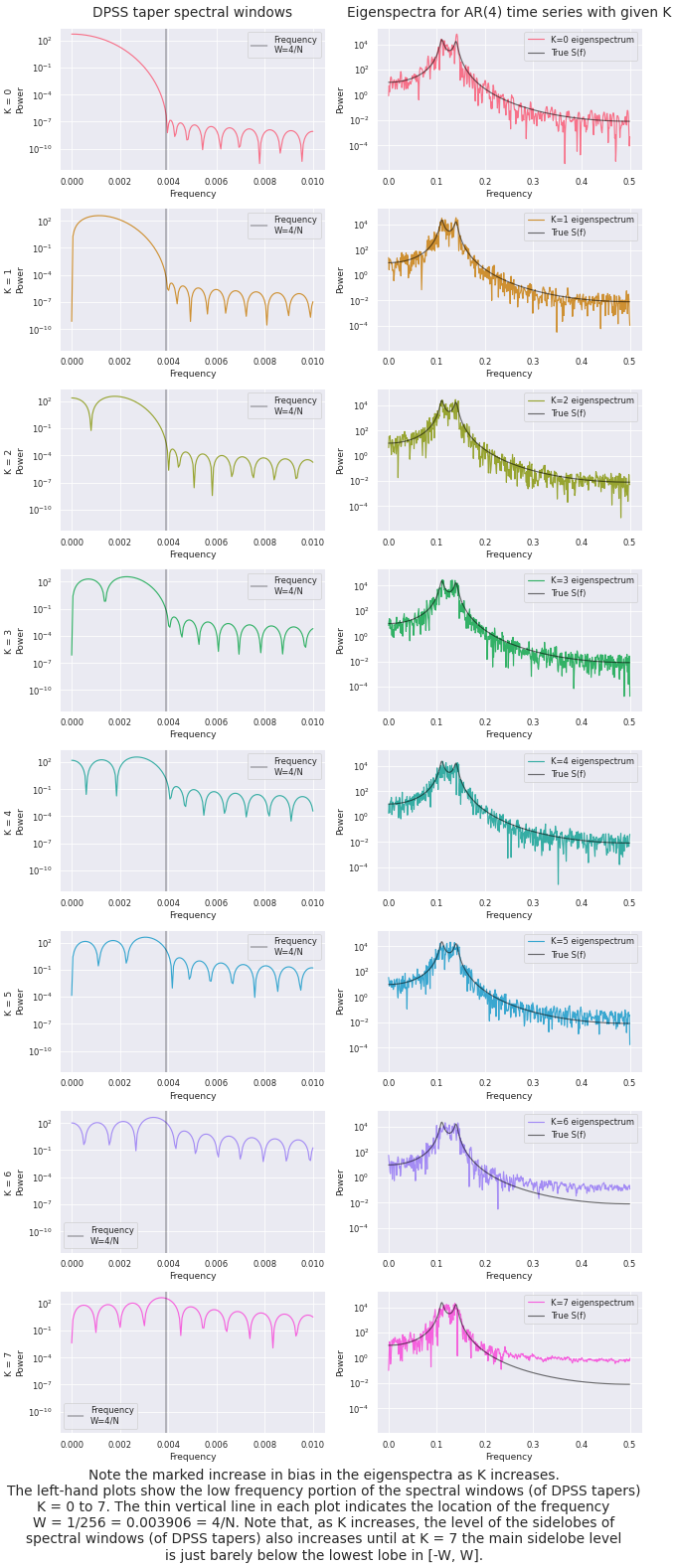
For this example, we took the normalized half-bandwidth product to be equal to 4 (NW = 4), resulting in 8 tapers being used. The spectral concentration in the band [-W, W] can then be seen from the plots. (Here N, the number of data points, is 1024, hence, W = 4/N = 0.003906)

There is a significant increase in the bias of the PSD estimates as the spectral concentration of the tapers worsens. To prevent these estimates with greater biases from affecting the final averaged estimate but still use the variance reductions they bring, we weigh the different estimates according to their spectral concentration (percentage of energy concentrated in the desired frequency band).

This can be kicked up a notch by using what is called adaptive weighing, which adaptively (duh?!) combines the different estimates, calculating the weights using an iterative process.

A brief summary of the Multitaper spectral estimation

https://medium.com/media/3f23eb5c2c41460b8793fbc2e6fbc04d/href

This summary, by no means, is an exhaustive explanation of the multitapering concept. Further exploration of the topic is highly encouraged. Use the references as the starting point.

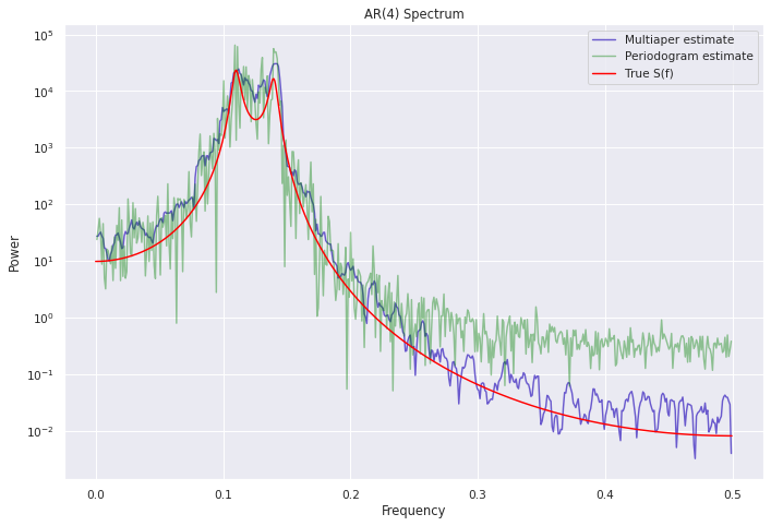
The Final Result

Using all the techniques outlined here, let's see how well can this multitaper periodogram estimate the true spectrum of this auto-regressive process. Also added is the classical periodogram (also sometimes referred to as a naïve spectrum estimator because of its basic estimation process) for comparison.

Here the multitaper estimate uses the adaptive weighting technique and the first 7 DPSS tapers

All this functionality is now implemented in Stingray²

References

[1]: Springford, Aaron, Gwendolyn M. Eadie, and David J. Thomson. 2020. “Improving the Lomb–Scargle Periodogram with the Thomson Multitaper.” The Astronomical Journal (American Astronomical Society) 159: 205. doi:10.3847/1538–3881/ab7fa1.

[2]: Huppenkothen, Daniela, Matteo Bachetti, Abigail L. Stevens, Simone Migliari, Paul Balm, Omar Hammad, Usman Mahmood Khan, et al. 2019. “Stingray: A Modern Python Library for Spectral Timing.” The Astrophysical Journal (American Astronomical Society) 881: 39. doi:10.3847/1538–4357/ab258d.

[3]: Thomson, D. J. 1982. “Spectrum Estimation and Harmonic Analysis.” IEEE Proceedings 70: 1055–1096. https://ui.adsabs.harvard.edu/abs/1982IEEEP..70.1055T.

[4]: Slepian, D. 1978. “Prolate Spheroidal Wave Functions, Fourier Analysis, and Uncertainty-V: The Discrete Case.” Bell System Technical Journal (Institute of Electrical and Electronics Engineers (IEEE)) 57: 1371–1430. doi:10.1002/j.1538–7305.1978.tb02104.x

[5]: D.B. Percival and A.T. Walden, Spectral Analysis for Physical Applications: Multitaper and Conventional Univariate Techniques. Cambridge, U.K.: Cambridge Univ. Press, 1993.

[6]: Thomson, D. J. 1990. “Time series analysis of Holocene climate data.” Philosophical Transactions of the Royal Society of London. Series A, Mathematical and Physical Sciences (The Royal Society) 330: 601–616. doi:10.1098/rsta.1990.0041