**“Across the sea of space, the stars are other suns.”** ~ Carl Sagan

Firstly, I would like to apologize for not posting a blog for more than a month.

Secondly, I would again like to apologize as this blog is going to be astronomically jargon-heavy(pun intended).
Now before you decide to just watch the funny Joey video and go watch more Friends episodes; trust me after reading this 7 minute blog you will gain serious bragging rights. After which you can binge Friends to your heart’s content(I already got my popcorn bowl with me 😉).

Community Bonding Phase and APE — 17

**“Community is about doing something that makes belonging matter”**

Community, as defined by the Cambridge Dictionary is the “people living in one particular area or people who are considered as a unit because of their common interests, social group, or nationality.”

Akin to the communities in the real world, the Open-Source Software community is one of the most diverse and active communities in the world. All Open-Source projects from the Linux Kernel to a niche, newly conceptualized project have several contributors keeping the project alive.
The best part about this online community is that any individual willing to contribute to the project is welcomed irrespective of their caste, creed, gender, race, nationality, level of expertise.
To be a part of a community of zealous, like-minded individuals working towards making the world a better place with software, makes you feel somewhat like a superhero😁.

The power of Open-Source is the power of the people ~ Philippe Kahn

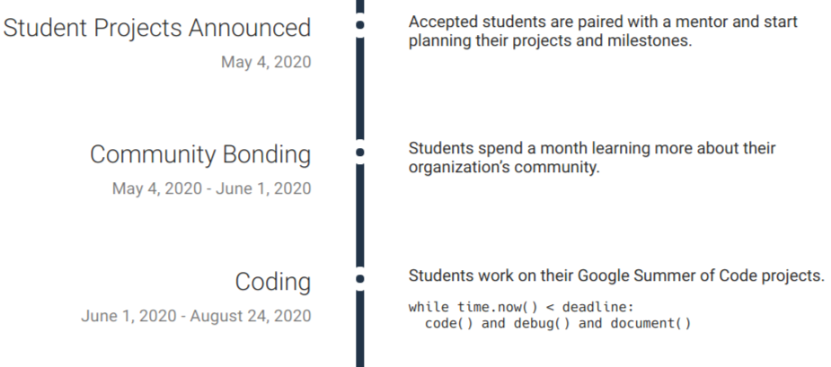
The community bonding phase is probably the most important part of the whole program. A month is given to students to get acquainted with the project community and mentors. Students are expected to get familiarized with the Code of Conduct and other guidelines such as Contributing, Coding, Testing guidelines.
This is an amazing opportunity to not only plan and research more about one’s project but also interact with other students of the same/different organization’s and learn more about their projects.

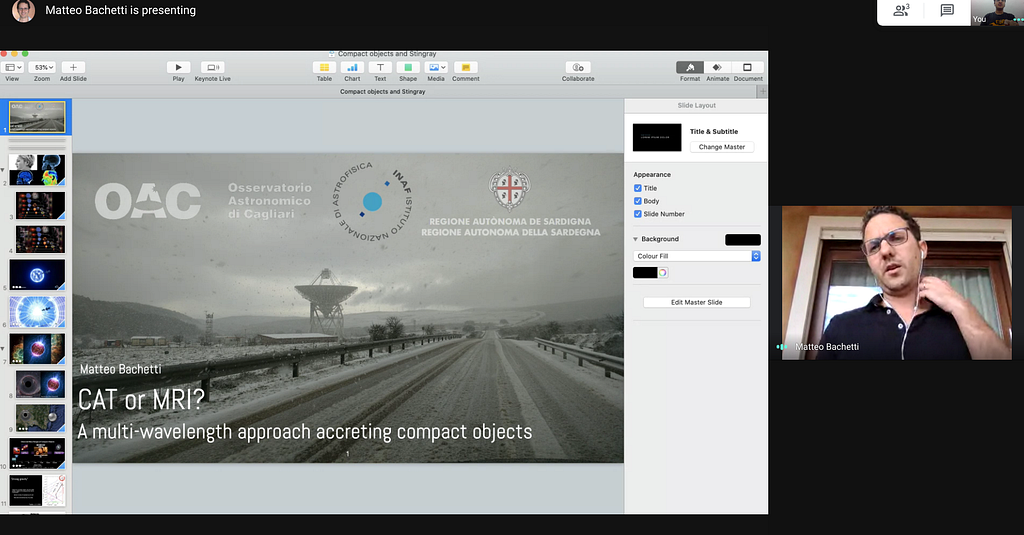
First Contact. The most exhilarating~2700 seconds of my life

I had two calls with my mentor Mr Matteo Bachetti during the community bonding phase. Lucky me, I got a one-to-one introduction to X-Ray Astronomy(with an amazing presentation) from Mr Bachetti himself!!
We discussed the goals, specifics as well as a rough trajectory of the project.

The community bonding phase gave me an amazing opportunity to not only associate with my peers from OpenAstronomy but also other organizations. I was particularly interested in a few projects from CERN-HSF as well as other projects from various sub-organizations in OpenAstronomy.
Thank you so much, Siddharth Lal, Biswarup Banerjee, Raahul Singh, Kris Stern, Abhijeet Manhas and Sahil Yadav, Honey Gupta, Prateek Kumar Agnihotri and Pranath Reddy for answering my persistent and often novice-level questions. You guys are awesome!!

Towards the end of the community bonding phase, I started working on updating stingray to APE-17(view my PR here). It was my first major PR(For all the non-techies out there a Pull Request(PR) is a proposal to implement changes to the main codebase to squash a bug or add a new feature). Looking at the status of the PR changed to “merged” gave me an unprecedented level of gratification. #justprogrammerthings
I will not bore you with the technical aspects of APE-17 but if you wish to learn more about it, here’s a summarized document I created.

X-ray Astronomy 101 with stingray

Disclaimer: I am not an expert at X-ray Astronomy, not even by a long shot(Just a month’s experience). I am a Computer Science techie, passionate about space and great at googling stuff 😁.

Now the part that all of you have been waiting for, the part that will give you the ultimate bragging rights of learning something new, being productive in these lazy lockdown times, presenting to you(insert drum roll)
X-ray Astronomy 101 with stingray.

1. What is stingray? What does it do?

Stingray is a community-developed spectral-timing software package in Python for astrophysical data. It provides a basis for advanced spectral-timing analysis with a correct statistical framework while also being open-source.
Stingray provides functionalities such as:
a. Constructing light curves from event data and performing various operations on light curves (e.g. add, subtract, join, truncate)
b. Good Time Interval operations
c. Creating periodograms(power spectra) and cross spectra
and many more.

2. So well what does all of this mean?

I apologize for the abrupt deep dive into the realm of long and daunting words that make zero sense at the moment. But please bear with me for a moment, once we are done with the basic you will truly appreciate the role that stingray plays.

So let’s start with the basics.

A time series is a simple graph that can be plotted for any values eg. temperature, rainfall, stock price etc.

a. Time Series: It is a sequence of observations recorded at a succession of time intervals. In general, time series are characterized by the interdependence of its values. This means that the value of the series at some time t is generally not independent of its value at, say, t−1.

b. Time Series Analysis: It is a statistical technique that deals with gaining insights from periodic or stochastic(a fancy way of saying random, aperiodic) time-series data.

Now let’s learn some astronomical terms:

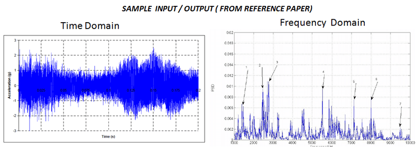
a. Timing Analysis: Many time series show periodic behaviour. This periodic behaviour can be very complex. Spectral analysis is a technique that allows us to discover underlying periodicities by decomposing the complex signal into simpler parts. To perform spectral analysis, we first must transform data from the time domain to the frequency domain.
Hence spectral analysis can be defined as decomposing a stationary time series {xT} into a combination of sinusoids(sine waves), with a random (and uncorrelated) coefficient; essentially analysis in the frequency domain.

b. Good Time Intervals (GTI’s): When observing a stellar object with a satellite, data is accumulated by observing the source with short exposures over time or collecting single photons(light particles) with their arrival time.
While recording observations, there will be times when everything is working perfectly. At other times we might have obstructions from the Earth that hinder our ability to observe the source properly.
Good time intervals (GTIs) are the time intervals where instruments are working well and the source is perfectly visible.

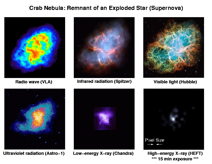
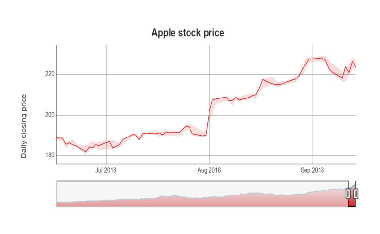
c. Light Curves: Light curves are graphs that show the brightness of an object over a period of time. Images show from the part of an object from where light is emitted. Another piece of information we have about light is the time when it reaches the detector. Astronomers use this “timing” information to create light curves and perform timing analysis.
They are simply graphs of brightness (Y-axis) vs. time (X-axis). Brightness increases as you go up the graph and time advances as you move to the right.
eg. The following lightcurve can be generated with the values from the table on the left. The change in brightness is periodic.

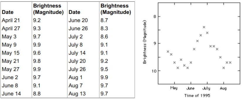
We can generate similar light curves for studying any part of the light spectrum eg. X-Rays. The record of changes in brightness that a light curve provides can help astronomers understand processes at work within the object they are studying and identify specific categories of stellar events.

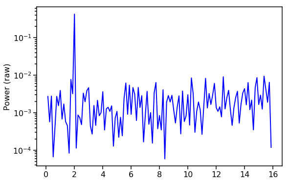
d. Spectral Density/Power Spectra: The power spectra of a time series {xT} describes the distribution of power into the frequency components of that signal. When these signals are viewed in the form of a frequency spectrum, certain aspects of the received signals or the underlying processes producing them are revealed.

e. Power Spectral Density Function: A Power spectral density function (PSD) shows the number of energy variations as a function of frequency. In other words, it shows at which frequencies are variations strong, weak.

f. Cross Spectra: Cross spectral analysis allows one to determine the relationship between two time-series as a function of frequency. Normally, we wish to compare two time-series along their peaks to see if these signals are related to one another at the same frequency and if so, what is the phase relationship between them. Even if two signals look identical we wish to check their periodicity and understand how they are related.
The Cross spectrum is a frequency domain analysis of the cross-correlation (how two lightcurves are related) or cross-covariance(how two lightcurves are related if one of them is linearly transformed eg. shifted in time).
For further reference check this out: https://atmos.washington.edu/~dennis/552_Notes_6c.pdf

3. How does stingray contribute to all of this confusing stuff?

Stingray implements all of these complex functions in a single easy to use package. It has various methods and classes such as lightcurve, powerspectrum, crossspectrum.
Stingray also provides a HENDRICS CLI and dave GUI interface for abstract analysis.

Woohoo!!🎉🎉 you made it through.
Now if all of this intrigues you as much as it did me, you can go through the references mentioned below and the stingray notebooks that demonstrate the functionality mentioned above or even fork the repository and tinker around with the code yourself(Highly Recommended!).

Thank you soo much for giving it a read. Please comment and leave a clap if you liked the article. Feel free to reach out to me on Linkedin.
Have an amazing day!! You are awesome!!!

References:

1. http://web.stanford.edu/class/earthsys214/notes/series.html
2. https://www.investopedia.com/terms/t/timeseries.asp
3. https://imagine.gsfc.nasa.gov/science/toolbox/timing1.html
4. http://coolwiki.ipac.caltech.edu/index.php/What_is_a_periodogram