My adventure with the implementation

While taking on this project, the thing I was most excited was that I would be getting to write rearch code (Code to be used by researchers in their work all over). With advent of large data from multiple telescopes and computational speed , Gaussian Processes are fast becoming the go to choice for astrophichal modelling.

In the original Source paper, the authors had simulated 1000 lightcurves of varying intesity of QPO, and measured their evidence for QPO and RN priors to check how well this technique works, and ensure that it does not give any false positives.

Hense, I set forth on my mission to calculate evidence of 1000 lightcurve on GPs with my new and beloved Macbook. Having full confidence that my computation machine is as good as they come, I set out to perform inference on my 1000 lightcurve, only for my pc to take 1 hour to without sampling a single lightcurve.

On reducing the number of points from 256 to 64, the code took 4 min to complete. Considering O(N3) time complexity, it would have taken 4 hours to complete the simulation for 1 curve :scream:.

Here I had made my own implementation of the kernel using tinygp. At this point my mentor advice me to use tinygp.quasisep.celerite kernels, a special kernel, implemented based on the celerite algorithm. On changing to the new kernel, the code took just 1 min to run. This made me realise how important such specialized code was, and how important making such faster and more effective code is.

The implementation

In the first two weeks I focussed on understanding the implementation of the project. In the source repository Celerite library was used for GP implimentation and Bilby was used for Bayesian Inferencing, while in my project my mentor and I decided to completely use a Jax based backend hense, Tinygp for GP, and Jaxns for Nested Sampling.

I made a proof of Concept implimentation for the QPO kernel and gaussian mean model for a lightcurve, which is explained in breif here:-

Kernel:

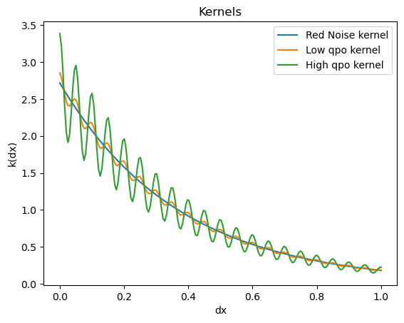
For making the Kernel, I used Tingp.quasisep.celerite kernels which are a fast implementation (based on the celerite kernel) of the Qpo kernel.

The quasisep.exp kernel for the red noise part and the quasisep.celerite kernel for the qpo part can be implemented as:

hqpokernel = kernels.quasisep.Exp(
scale = 1/hqpoparams["crn"], sigma = (hqpoparams["arn"])**0.5) + kernels.quasisep.Celerite(
a = hqpoparams["aqpo"], b = 0.0, c = hqpoparams["cqpo"], d = 2*jnp.pi*hqpoparams["freq"])

Plot of High, low and non QPO kernel

Mean:

We are working on Extremely powerful events in the universe which emit radiation in the Xray spectra. Many of these have some sort of flaring behaviour, and also in general, we wanted to add mean functions to our GPs as this feature will be extended to other astronomical time series.

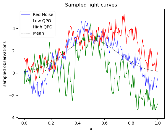
For this proof of concept implimentation, I used a simple gaussian mean to test out sampling using Jaxns Using the tinygp library to make the gaussian process and sample out some lightcurves from it.

def gaussian(t, mean_params):
return mean_params["A"] * jnp.exp(-((t - mean_params["t0"])**2)/(2*(mean_params["sig"]**2)))

mean_params = {
"A" : 3,    "t0" : 0.5,    "sig" : 0.2,}

mean = functools.partial(gaussian, mean_params = mean_params)
# Making the Gp
gp = tinygp.GaussianProcess( kernel, t, mean=mean, diag = diag)
gp_sample   =  gp.sample( jax.random.PRNGKey(11), shape=(1,))

Plot of samples

Priors and likelihoods

As we want to fit our Red noise and Qpo + Red noise model on the lightcurve, we need to make suitable prior funcitons for them. We use Jaxns.Prior to make a generator prior function, and make a corresponding likelihood function, which makes the gp and calculates the log likehood of producing the given lightcurve.

We set the bounds for the prior functions based on the suggestions given in the source paper, and plot the fitted maximum posterior gp on the lightcurve.

# Prior Model Function
def RNprior_model():
T = Times[-1] - Times[0]    # Total time
    f = 1/(Times[1] - Times[0]) # Sampling frequency
    min = jnp.min(lightcurve); max = jnp.max(lightcurve)
span = max - min

# Red noise kernel prior
    arn = yield Prior(tfpd.Uniform(0.1*span, 2*span), name='arn')
crn = yield Prior(tfpd.Uniform(jnp.log(1/T), jnp.log(f)), name='crn')

# Gaussian mean priors
    A = yield Prior(tfpd.Uniform(0.1*span, 2*span), name='A')
t0 = yield ForcedIdentifiability(n = 1, low = Times[0]-0.1*T, high = Times[-1]+0.1*T, name='t0')
sig = yield Prior(tfpd.Uniform(0.5*1/f, 2*T), name='sig')
return arn, crn, A, t0, sig

# Log Likelihood Function
@jit
def RNlog_likelihood2(arn, crn, A, t0, sig):
rnlikelihood_params = {"arn": arn, "crn": crn,
"aqpo": 0.0, "cqpo": 0.0, "freq": 0.0, }

mean_params = { "A": A, "t0": t0, "sig": sig, }

gp = build_gp(rnlikelihood_params, mean_params, Times, kernel_type = "RN")
return gp.log_probability(lightcurve)

# Nested Sampling using Jaxns
RNmodel = Model(prior_model= RNprior_model, log_likelihood=RNlog_likelihood2)
RNexact_ns = ExactNestedSampler(RNmodel, num_live_points= 500, max_samples= 1e4)
RNtermination_reason, RNstate = RNexact_ns(random.PRNGKey(42), term_cond=TerminationCondition(live_evidence_frac=1e-4))
RNresults = RNexact_ns.to_results(RNstate, RNtermination_reason)

Plot of samples

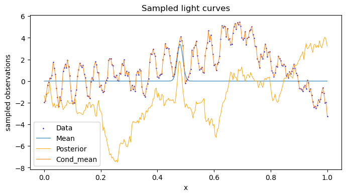
But the main use is not just to fit a GP, but rather to acess whether it contains a QPO or not. For that, we compare the evidence (Bayes Factor) of the lightcurve for a QPO_RN Gp and RN GP, and as expected, for a high QPO sample, we get a high value of (-212 - (-262)) = 50.

The image in the top is of the QPO model sampling.

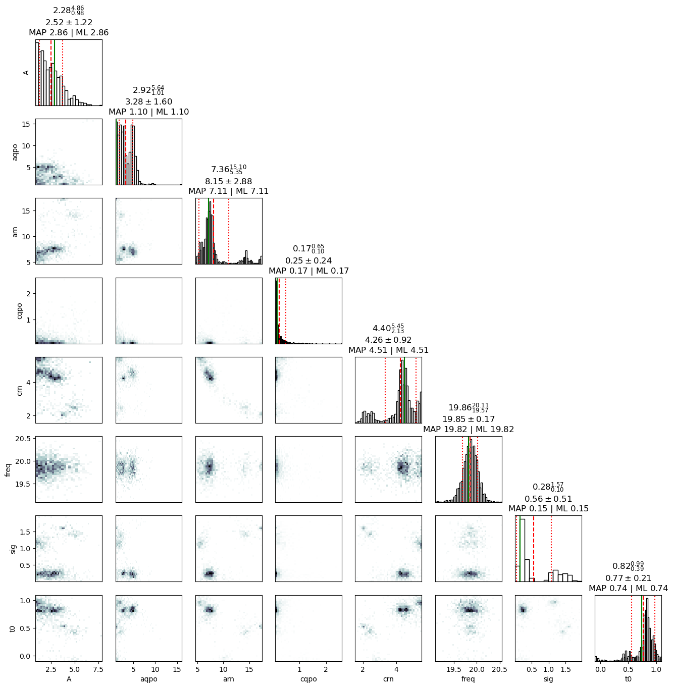
The corner plot shows the result of the sampling, and the frequency of 20Hz is captured well in it.

Plot of samples

Tensor flow probability

TensorFlow Probability (TFP) is a Python library built on TensorFlow that makes it easy to combine probabilistic models and deep learning on modern hardware (TPU, GPU).

For this project, the jax backend requires that we also use tfpd to make our priors, and as I had to use some joint priors I explored the library.

The joint priors could not be integrated with jaxns sampling, as multi-parameter priors lacked quantiles, but it was time well spent, as I was able to see a powerful library which had almost all kinds of priors and inferencing techniques under the sky, while supporting its own implementaions of NUTS and MCMC sampling.